Quantum Chromodynamics 2026, 03 - MIT Bag Model
The most common model of quark-quark interaction is an SU(3) gauge theory, including colour-interaction as its d.o.f. The accuracy of calculation are fairly low (4.0). I at this point presuppose knowledge of the gauge theory underlying the standard model that the book sketches in chapter 4.1.
A gauge theory for quark-quark interactions requires knowledge of the number of "charge states" for the colour interaction. In high-energy e+e- reactions hadrons are created by pair annihilation, then quark-antiquark pairs are created. By asymptotic freedom, the interaction doesn't influence the cross section. The creation of quark-antiquark pairs is analogous to that of other particle-antiparticle pairs (p. 165). The calculation of the R-factor provides arguments for the number of colours being 3. For all energy regimes, this factor should scale linearly with that number, and comparing these with experimental data sets this number (p. 166 - 167). All theories for quark-quark interactions has to start with 3 colour states (p. 170). These can be mapped to the fundamental representation of the SU(3) colour group. This group is chose, because it's the only group with complex irreducible triplets. Alternatives to QCDs then must have at least a spontaneously broken SU(3) symmetry and some high mass residues of the original group (p. 170).
Quantum field theories are often subject to dimensional regularization. Other forms of regularization exist, but are applied more selectively (p. 184). Dimensional regularization emerges from the observation that only standard QFTs only encounter log-divergences, which vanish for dimensionalities smaller than 4. They can then by isolated by defining generalized integration for noninteger dimensions d with divergences d - 4. The standard tool for this is the Wick rotation. A divergent integral of QFT has the general form

(Eq. 4.59). For large kμ, this integral is non-uniform, as k2 can stay small, even for large components. To circumvent, this, rotate the 0-component of k into imaginary space, and leaving the spatial components in real space (p. 185). To counter the change, the integration path needs to be deformed in the 0-component, to rotate it into the complex plane. This enters the integrals into residuum computation, of which the non-defined cases can be set to zero (Eq. 4.60). This can be generalized to a d-dimensional integral ∫dd kE f(kE) (p. 186). This operation is linear, invariant under finite shifts and scales inversely (Eqs. 4.64 - 66).
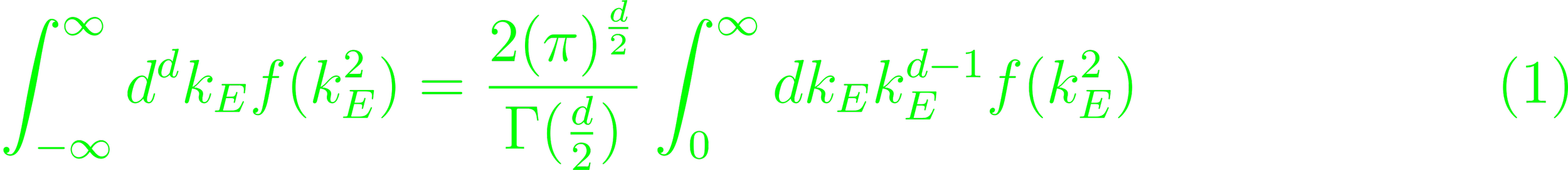
(Eq. 4.71c). All integrals can be expanded as a sum of Gaussians, which enables direct d-integration.
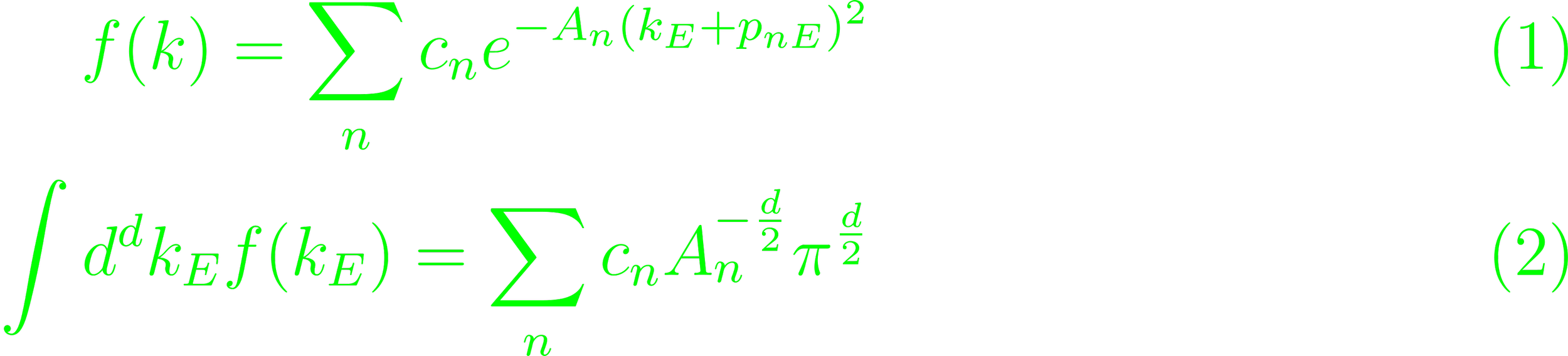
(Eqs. 4.74, 4.71d). This sum doesn't necessarily converge. For divergent integrals, the sum doesn't converge (p. 191).