Loops, Knots, Gauge Theories and Quantum Gravity 2026, 24 - Loop and Bargman Representation

For a Loop representation from the Maxwell case, choose a polarization in which wavefunctions are functionals of the connection Ψ[A] for both chosen Maxwell parameters, and extrapolate to Gauss law

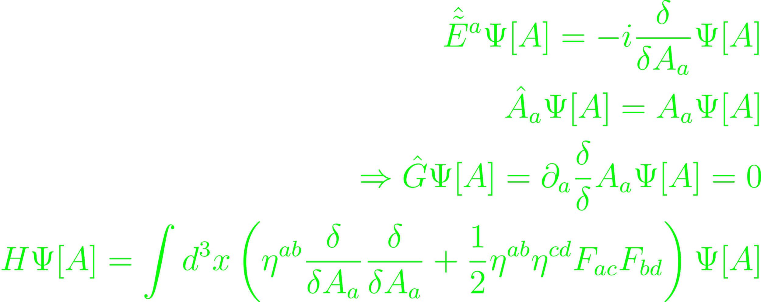
(Eqs. 4.48 - 51) which implies that Ψ[A] is gauge invariant. The loop representation in the Abelian case immediately determines a non-canonical algebra of gauge invariant operators. For the non-Abelian case, the familiar T operators are required, along with the non-canonical algebra (Eqs. 4.52 - 58). The loop transform follows

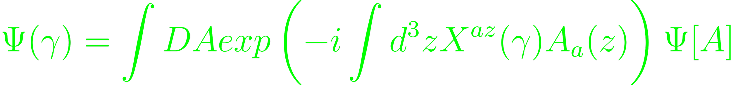
The natural intepretation of loops in loop represenation are lines of electric flux (p. 98) through the loop transform.

(Eqs. 4.66 - 69). Through these, the Hamiltonian can be expressed through loops.

(Eq. 4.72). The eigenvalue equation is functionally the same as the Laplacian in terms of the double loop derivative. The expression for the eigenstates follow directly (4.4).

The canonical formulation of the harmonic oscillator follows the typical Hamiltonian in generalized position and momentum operators, and the resulting eigenvalue equation. The complex coordinatization is also standard. The operational relations determine the inner product, which can be first assumed to be the generic inner product. Using the circular polarization for the electric and gauge fields, both create a conjugate pair which expresses the degrees of freedom for the Maxwell field through the complex field ζ(k)_i = 2^-1/2(|k|q_i^(c)(k) - ip_i^(c)(k)) (p. 105). Their commutation relation defines their quantization as quantum operators

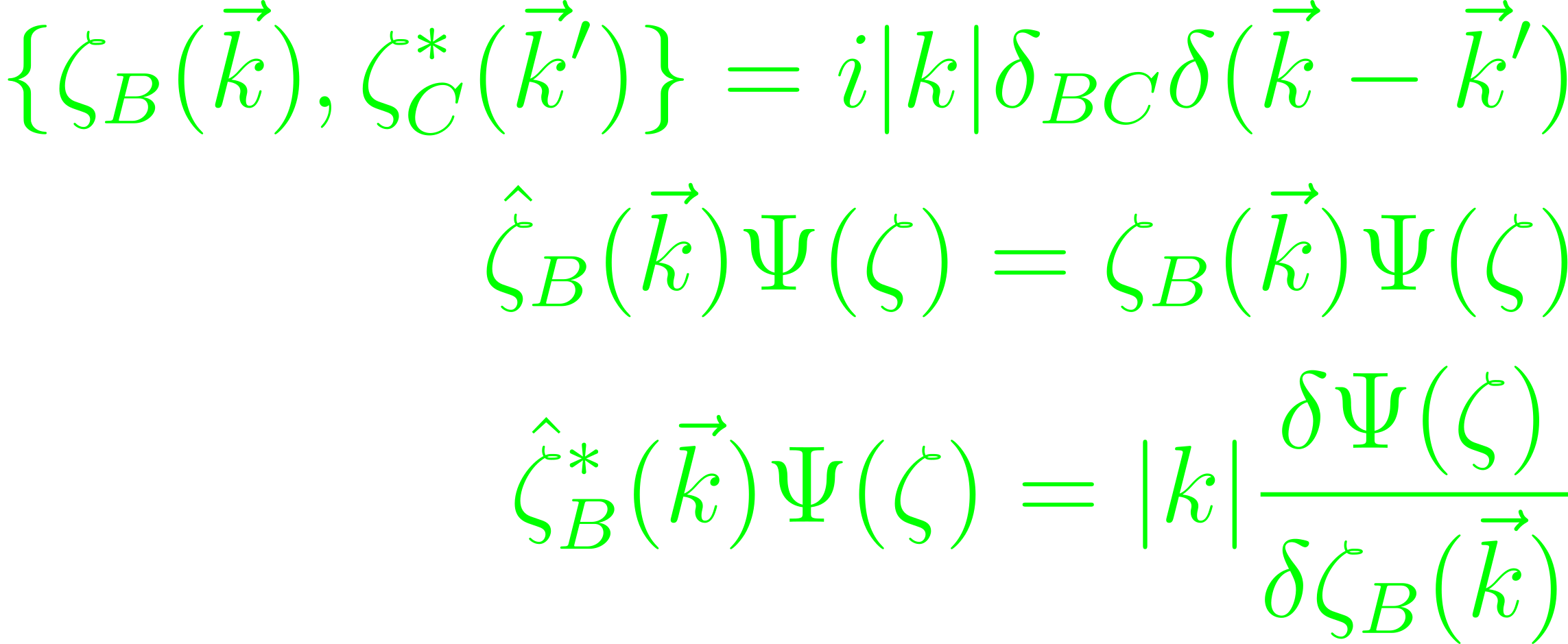
(Eq. 4.114 - 116). With the inner product, the Gaussian measure can be set

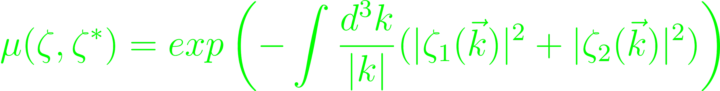
(Eq. 4.120). The ground state Ψ(ζ) = 1 follows directly from the normal-ordered Hamiltonian. This quantization is problematic, because the inner product in terms of loops features a non-trivial Gauss-measure which is considered ill-defined.