Convex Optimization 2026, 26 - Parametric Distribution Estimation

A family of probability distributions indexed by vectors x with densities p_x can define p_x(y) as likelihood functions (which implicitly defines the log-likelihood functions l(x) = log p_x(y)). Constraints on x representing prior knowledge about the event x or the domain of the likelihood function can be explicitly given or incorporated into the likelihood function. Estimating the value of x based on a sample y from the distribution is usually done through maximum likelihood estimation (ML). It maximizes l(x), while x ∈ C (Eq. 7.1). A linear measurement model y_i = a_i^Tx + v_i where x is a vector of parameters to be estimated and v is the noise, which is assumed independently, identically distributed with density p, the likelihood functions are

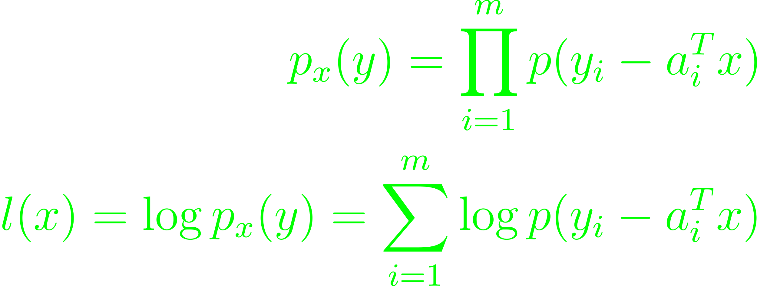
The ML estimates are optimal points for the problem maximizing l(x) (Eq. 7.2). Penalty function approximation problems minimizing ∑^m_i=1ϕ(b_i - a_i^Tx) can be written as maximum likelihood estimation problem with noise density. If the random variable y is integer valued with a Poisson distribution, the problem qualifies as a counting problem with the mean μ = a^Tu + b where the vector u is made from explanatory variables. Given a gaussian random variable with zero mean and covariance matrix R = E yy^T with density p_R(y) = (2π)^-n/2det(R)^-1/2exp(-y^TR^-1y/2); R ∈ Sⁿ₊₊. The covariance matrix R is estimated off N independent samples drawn from the distribution. Then, with the sample covariance Y

Using the inverse covariance matrix S instead, l(S) becomes a concave function in S, so the ML estimate of S maximizes log det S - tr(SY) (7.1.1).

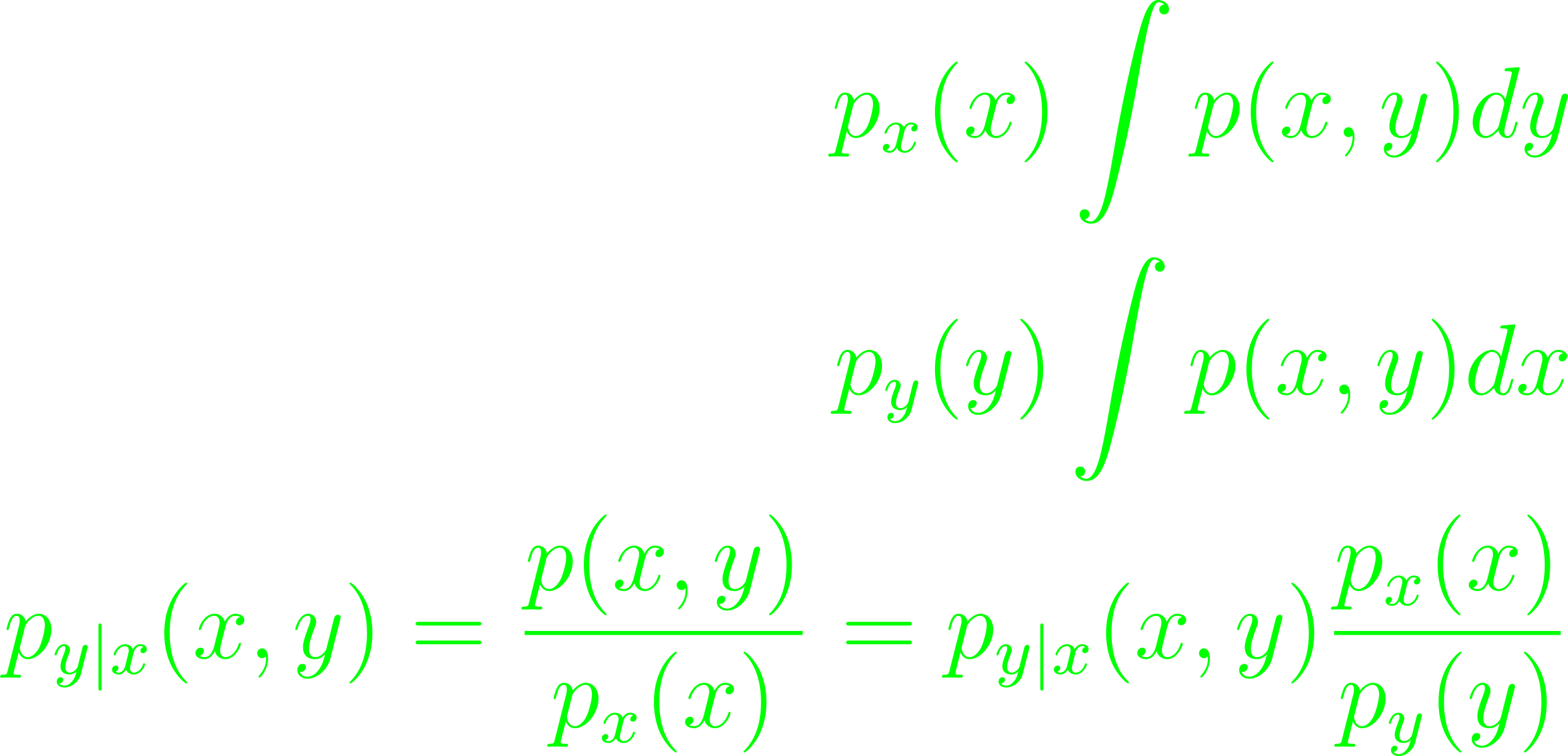
Maximum a posteriori probability (MAP) estimation is Bayesian version of maximum likelihood. Given prior densities p_x, p_y and define the conditional density p_y|x(x, y)

Given some IID noise v_i, the MAP estimates are determined by minimizing (x - x)^T∑^-1(x - x') under the inf-norm (7.2).