Convex Optimization 2026, 12 - Linear Optimization Problems

Quadratic optimization problems minimize (1/2)x^TPx + q^Tx + r so that Gx ⪯ h, Ax = b where P ∈ Sⁿ₊, G ∈ ℝ^{m × n}, A ∈ ℝ^{p × n}. This is a quadratic program (p. 152). If additionally, the inequality constraint functions are quadratic, then it's a quadratically constrained quadratic program (QCQP). In such a program, the convex quadratic function is minimized over feasible regions that are intersections of ellipsoids. Technically, linear programs are a special case of this problem (P = 0) (p. 153).

Closely related is the second-order cone program (SOCP), which minimizes f^Tx with ||A_ix + b_i||₂ ≤ c_i^Tx + d_i, Fx = g. These constraints are second-order cone constraints and generalizes an affine function into multiple dimensions (4.4.2).

Given a linear program in inequality form with some variation in its constraint parameters (and function parameters). Fixing two of these for any given constraint will place the remaining one into ellipsoid sets. Requiring that the constraint be satisfied for all possible values for such a parameter defines the robust linear program. The robust linear program can be mapped into a statistical framework (4.4.2.2).

The surface area of a graph of a function f with dom f = C is a convex functional of f.

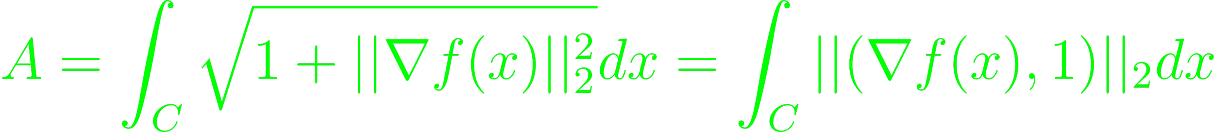
The minimal surface problem is to find f minimizing A, with additional constraints. The problem can be approximated by discretizing f (4.4.2.3).

A monomial function is of the form f(x) = cΠi=1nxiia where c > 0 and ai ∈ ℝ. A sum of such monomials are posynomial functions. They are closed under addition, multiplication and nonnegative scaling. Monomials are closed under multiplication and division (4.5.1).

A geometric program is an optimization problem minimizing f(x)₀ with f(x)_i ≤ 1, h_i(x) = 1. It can be extended to posynomial f and monomial h, in which case the constraint f(x) ≤ h(x) being handled by the posynomial f(x)/h(x) ≤ 1, similarly, if f(x) ≤ a, a > 0. Also similarly, if h₁(x) = h₂(x) ⇒ h₁/h₂ = 1 (4.5.2). Geometric programs are not generally convex optimization problems, but can be transformed into one by change of variables and transforming the objective and constraint functions (4.5.3).